Bilješka
Pristup ovoj stranici zahtijeva provjeru vjerodostojnosti. Možete pokušati da se prijavite ili promijenite direktorije.
Pristup ovoj stranici zahtijeva provjeru vjerodostojnosti. Možete pokušati promijeniti direktorije.
Automated Machine Learning (AutoML) includes techniques and tools that streamline the process of training and optimizing machine learning models with minimal human intervention. AutoML simplifies and accelerates the selection of the most suitable machine learning model and hyperparameters for a given dataset. This task typically requires considerable expertise and computational resources. Within the Fabric framework, data scientists can use the flaml.AutoML module to automate various aspects of their machine learning workflows.
In this article, you learn how to generate AutoML trials directly from code by using a Spark dataset. You also learn how to convert this data into a Pandas dataframe and how to parallelize your experimentation trials.
Prerequisites
Get a Microsoft Fabric subscription. Or, sign up for a free Microsoft Fabric trial.
Sign in to Microsoft Fabric.
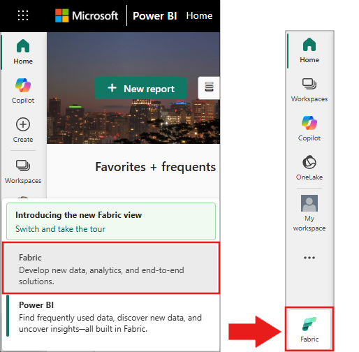
Switch to Fabric by using the experience switcher on the lower-left side of your home page.
- Create a new Fabric environment or ensure you're running on Fabric Runtime 1.3 (Spark 3.5 and Delta 3.2) or higher. For the full list of supported runtimes, see Apache Spark runtimes in Fabric.
- Create a new notebook.
- Attach your notebook to a lakehouse. On the left side of your notebook, select Add to add an existing lakehouse or create a new one.
Load and prepare data
In this section, you specify the download settings for the data and then save it to the lakehouse.
Download data
This code block downloads the data from a remote source and saves it to the lakehouse.
import os
import requests

IS_CUSTOM_DATA = False  # if TRUE, dataset has to be uploaded manually

if not IS_CUSTOM_DATA:
    # Specify the remote URL where the data is hosted
    remote_url = "https://synapseaisolutionsa.z13.web.core.windows.net/data/bankcustomerchurn"

    # List of data files to download
    file_list = ["churn.csv"]

    # Define the download path within the lakehouse
    download_path = "/lakehouse/default/Files/churn/raw"

    # Check if the lakehouse directory exists; if not, raise an error
    if not os.path.exists("/lakehouse/default"):
        raise FileNotFoundError("Default lakehouse not found. Please add a lakehouse and restart the session.")

    # Create the download directory if it doesn't exist
    os.makedirs(download_path, exist_ok=True)

    # Download each data file if it doesn't already exist in the lakehouse
    for fname in file_list:
        if not os.path.exists(f"{download_path}/{fname}"):
            r = requests.get(f"{remote_url}/{fname}", timeout=30)
            with open(f"{download_path}/{fname}", "wb") as f:
                f.write(r.content)

    print("Downloaded demo data files into lakehouse.")
Load data into a Spark dataframe
The following code block loads the data from the CSV file into a Spark DataFrame and caches it for efficient processing.
df = (
    spark.read.option("header", True)
    .option("inferSchema", True)
    .csv("Files/churn/raw/churn.csv")
    .cache()
)
This code assumes that you downloaded the data file and that it's located in the specified path. It reads the CSV file into a Spark DataFrame, infers the schema, and caches it for faster access during subsequent operations.
Prepare the data
In this section, you clean the data and perform feature engineering on the dataset.
Clean data
First, define a function to clean the data. The function drops rows with missing data, removes duplicate rows based on specific columns, and drops unnecessary columns.
# Define a function to clean the data
def clean_data(df):
    # Drop rows with missing data across all columns
    df = df.dropna(how="all")
    # Drop duplicate rows based on 'RowNumber' and 'CustomerId'
    df = df.dropDuplicates(subset=['RowNumber', 'CustomerId'])
    # Drop columns: 'RowNumber', 'CustomerId', 'Surname'
    df = df.drop('RowNumber', 'CustomerId', 'Surname')
    return df

# Create a copy of the original dataframe by selecting all the columns
df_copy = df.select("*")

# Apply the clean_data function to the copy
df_clean = clean_data(df_copy)
The clean_data function ensures the dataset is free of missing values and duplicates while removing unnecessary columns.
Feature engineering
Next, perform feature engineering by creating dummy columns for the Geography and Gender columns using one-hot encoding.
# Import PySpark functions
from pyspark.sql import functions as F

# Create dummy columns for 'Geography' and 'Gender' using one-hot encoding
df_clean = df_clean.select(
    "*",
    F.when(F.col("Geography") == "France", 1).otherwise(0).alias("Geography_France"),
    F.when(F.col("Geography") == "Germany", 1).otherwise(0).alias("Geography_Germany"),
    F.when(F.col("Geography") == "Spain", 1).otherwise(0).alias("Geography_Spain"),
    F.when(F.col("Gender") == "Female", 1).otherwise(0).alias("Gender_Female"),
    F.when(F.col("Gender") == "Male", 1).otherwise(0).alias("Gender_Male")
)

# Drop the original 'Geography' and 'Gender' columns
df_clean = df_clean.drop("Geography", "Gender")
Use one-hot encoding to convert categorical columns into binary dummy columns, making them suitable for machine learning algorithms.
Display cleaned data
Finally, display the cleaned and feature-engineered dataset by using the display function.
display(df_clean)
This step lets you inspect the resulting DataFrame with the applied transformations.
Save to lakehouse
Now, save the cleaned and feature-engineered dataset to the lakehouse.
# Create PySpark DataFrame from Pandas
df_clean.write.mode("overwrite").format("delta").save(f"Tables/churn_data_clean")
print(f"Spark dataframe saved to delta table: churn_data_clean")
Here, take the cleaned and transformed PySpark DataFrame, df_clean, and save it as a Delta table named churn_data_clean in the lakehouse. Use the Delta format for efficient versioning and management of the dataset. The mode("overwrite") option ensures that any existing table with the same name is overwritten, and a new version of the table is created.
Create test and training datasets
Next, create the test and training datasets from the cleaned and feature-engineered data.
In the provided code section, load a cleaned and feature-engineered dataset from the lakehouse using Delta format, split it into training and testing sets with an 80-20 ratio, and prepare the data for machine learning. This preparation involves importing the VectorAssembler from PySpark ML to combine feature columns into a single "features" column. Later, use the VectorAssembler to transform the training and testing datasets, resulting in train_data and test_data DataFrames that contain the target variable "Exited" and the feature vectors. These datasets are now ready for use in building and evaluating machine learning models.
# Import the necessary library for feature vectorization
from pyspark.ml.feature import VectorAssembler

# Load the cleaned and feature-engineered dataset from the lakehouse
df_final = spark.read.format("delta").load("Tables/churn_data_clean")

# Train-Test Separation
train_raw, test_raw = df_final.randomSplit([0.8, 0.2], seed=41)

# Define the feature columns (excluding the target variable 'Exited')
feature_cols = [col for col in df_final.columns if col != "Exited"]

# Create a VectorAssembler to combine feature columns into a single 'features' column
featurizer = VectorAssembler(inputCols=feature_cols, outputCol="features")

# Transform the training and testing datasets using the VectorAssembler
train_data = featurizer.transform(train_raw)["Exited", "features"]
test_data = featurizer.transform(test_raw)["Exited", "features"]
Train baseline model
Using the featurized data, train a baseline machine learning model, configure MLflow for experiment tracking, define a prediction function for metrics calculation, and finally, view and log the resulting ROC AUC score.
Set logging level
Here, configure the logging level to suppress unnecessary output from the Synapse.ml library, keeping the logs cleaner.
import logging

logging.getLogger('synapse.ml').setLevel(logging.ERROR)
Configure MLflow
In this section, configure MLflow for experiment tracking. Set the experiment name to "automl_sample" to organize the runs. Additionally, enable automatic logging, ensuring that model parameters, metrics, and artifacts are automatically logged to MLflow.
import mlflow

# Set the MLflow experiment to "automl_sample" and enable automatic logging
mlflow.set_experiment("automl_sample")
mlflow.autolog(exclusive=False)
Train and evaluate the model
Finally, train a LightGBMClassifier model on the provided training data. Configure the model with the necessary settings for binary classification and imbalance handling. Use this trained model to make predictions on the test data. Extract the predicted probabilities for the positive class and the true labels from the test data. Afterward, calculate the ROC AUC score by using sklearn's roc_auc_score function.
from synapse.ml.lightgbm import LightGBMClassifier
from sklearn.metrics import roc_auc_score

# Assuming you have already defined 'train_data' and 'test_data'

with mlflow.start_run(run_name="default") as run:
    # Create a LightGBMClassifier model with specified settings
    model = LightGBMClassifier(objective="binary", featuresCol="features", labelCol="Exited", dataTransferMode="bulk")

    # Fit the model to the training data
    model = model.fit(train_data)

    # Get the predictions
    predictions = model.transform(test_data)

    # Extract the predicted probabilities for the positive class
    y_pred = predictions.select("probability").rdd.map(lambda x: x[0][1]).collect()

    # Extract the true labels from the 'test_data' DataFrame
    y_true = test_data.select("Exited").rdd.map(lambda x: x[0]).collect()

    # Compute the ROC AUC score
    roc_auc = roc_auc_score(y_true, y_pred)

    # Log the ROC AUC score with MLflow
    mlflow.log_metric("ROC_AUC", roc_auc)

    # Print or log the ROC AUC score
    print("ROC AUC Score:", roc_auc)
From here, you can see that the resulting model achieves a ROC AUC score of 84%.
Create an AutoML trial with FLAML
In this section, create an AutoML trial by using the FLAML package, configure the trial settings, convert the Spark dataset to a Pandas on Spark dataset, run the AutoML trial, and view the resulting metrics.
Configure the AutoML trial
Import the necessary classes and modules from the FLAML package and create an instance of AutoML. Use this instance to automate the machine learning pipeline.
# Import the AutoML class from the FLAML package
from flaml import AutoML
from flaml.automl.spark.utils import to_pandas_on_spark

# Create an AutoML instance
automl = AutoML()
Configure settings
Define the configuration settings for the AutoML trial.
# Define AutoML settings
settings = {
    "time_budget": 250,         # Total running time in seconds
    "metric": 'roc_auc',       # Optimization metric (ROC AUC in this case)
    "task": 'classification',  # Task type (classification)
    "log_file_name": 'flaml_experiment.log',  # FLAML log file
    "seed": 41,                # Random seed
    "force_cancel": True,      # Force stop training once time_budget is used up
    "mlflow_exp_name": "automl_sample"      # MLflow experiment name
}
Convert to Pandas on Spark
To run AutoML with a Spark-based dataset, convert it to a Pandas on Spark dataset by using the to_pandas_on_spark function. This conversion enables FLAML to work with the data efficiently.
# Convert the Spark training dataset to a Pandas on Spark dataset
df_automl = to_pandas_on_spark(train_data)
Run the AutoML trial
Now, run the AutoML trial. Use a nested MLflow run to track the experiment within the existing MLflow run context. The AutoML trial runs on the Pandas on Spark dataset (df_automl) with the target variable Exited. Pass the defined settings to the fit function for configuration.
'''The main flaml automl API'''

with mlflow.start_run(nested=True):
    automl.fit(dataframe=df_automl, label='Exited', isUnbalance=True, **settings)
View resulting metrics
In this final section, retrieve and display the results of the AutoML trial. These metrics provide insights into the performance and configuration of the AutoML model on the given dataset.
# Retrieve and display the best hyperparameter configuration and metrics
print('Best hyperparameter config:', automl.best_config)
print('Best ROC AUC on validation data: {0:.4g}'.format(1 - automl.best_loss))
print('Training duration of the best run: {0:.4g} s'.format(automl.best_config_train_time))
Parallelize your AutoML trial with Apache Spark
In scenarios where your dataset can fit into a single node and you want to use the power of Spark for running multiple parallel AutoML trials simultaneously, follow these steps:
Convert to Pandas dataframe
To enable parallelization, first convert your data into a Pandas DataFrame.
pandas_df = train_raw.toPandas()
Here, convert the train_raw Spark DataFrame into a Pandas DataFrame named pandas_df to make it suitable for parallel processing.
Configure parallelization settings
Set use_spark to True to enable Spark-based parallelism. By default, FLAML launches one trial per executor. You can customize the number of concurrent trials by using the n_concurrent_trials argument.
settings = {
    "time_budget": 250,           # Total running time in seconds
    "metric": 'roc_auc',         # Optimization metric (ROC AUC in this case)
    "task": 'classification',    # Task type (classification)
    "seed": 41,                  # Random seed
    "use_spark": True,           # Enable Spark-based parallelism
    "n_concurrent_trials": 3,    # Number of concurrent trials to run
    "force_cancel": True,        # Force stop training once time_budget is used up
    "mlflow_exp_name": "automl_sample"  # MLflow experiment name

}
In these settings, specify that you want to utilize Spark for parallelism by setting use_spark to True. Set the number of concurrent trials to 3, meaning that three trials run in parallel on Spark.
To learn more about how to parallelize your AutoML trails, visit the FLAML documentation for parallel Spark jobs.
Run the AutoML trial in parallel
Now, run the AutoML trial in parallel with the specified settings. Use a nested MLflow run to track the experiment within the existing MLflow run context.
'''The main FLAML AutoML API'''
with mlflow.start_run(nested=True, run_name="parallel_trial"):
    automl.fit(dataframe=pandas_df, label='Exited', **settings)
This process executes the AutoML trial with parallelization enabled. Set the dataframe argument to the Pandas DataFrame pandas_df, and pass other settings to the fit function for parallel execution.
View metrics
After running the parallel AutoML trial, retrieve and display the results, including the best hyperparameter configuration, ROC AUC on the validation data, and the training duration of the best-performing run.
''' retrieve best config'''
print('Best hyperparmeter config:', automl.best_config)
print('Best roc_auc on validation data: {0:.4g}'.format(1-automl.best_loss))
print('Training duration of best run: {0:.4g} s'.format(automl.best_config_train_time))